[1]:

import matplotlib.pyplot as plt
import straph as sg
import numpy

                        

[2]:

plt.rcParams["figure.figsize"] = (12,9)

                        

In this section we will show how to use different methods, implemented in Straph, to generate random stream graphs.

Stream Graph Generators¶

Firstly, we must precise that the following methods may not be as intuitive as methods for random static graphs (Barabasi-Albert, Erdos-Renyi) but they are an adaptation for stream graphs. The addition of a temporal dimension, continuous by nature, necessitate a mixture of continous random variable (coding nodes and links presence, for the temporal dimension) and discrete random variable (coding nodes and links occurence, for the structural dimension).

Our generators take the following parameters:

T: the time window of the stream graph
nb_nodes: number of nodes
occurence_param_node: Occurence of a node (discrete variable)
presence_param_node: Node presence (continuous variable)
occurence_param_link: Occurence of a link (discrete variable)
presence_param_link: Link presence (continuous variable)

Erdos Renyi¶

[3]:

T = [0, 100]
nb_node = 21
occurrence_law_node = 'poisson'
presence_law_node = 'uniform'

occurrence_param_node = 3
presence_param_node = 25

occurrence_law_link = 'poisson'
presence_law_link = 'uniform'

occurrence_param_link = 5
presence_param_link = 15

                                

As for static graphs, this model takes a single parameter p_link which is the probability that two nodes are connected.

[4]:

p_link = numpy.sqrt(nb_node)/nb_node

                                

[5]:

S = sg.erdos_renyi(T,
                    nb_node,
                    occurrence_law_node,
                    occurrence_param_node,
                    presence_law_node,
                    presence_param_node,
                    occurrence_law_link,
                    occurrence_param_link,
                    presence_law_link,
                    presence_param_link,
                    p_link)
S.describe()

                                

Nb of Nodes :  21
Nb of segmented nodes :  38.0
Nb of links :  47
Nb of segmented links :  84.0
Nb of event times :  175

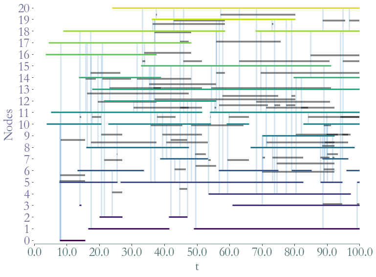
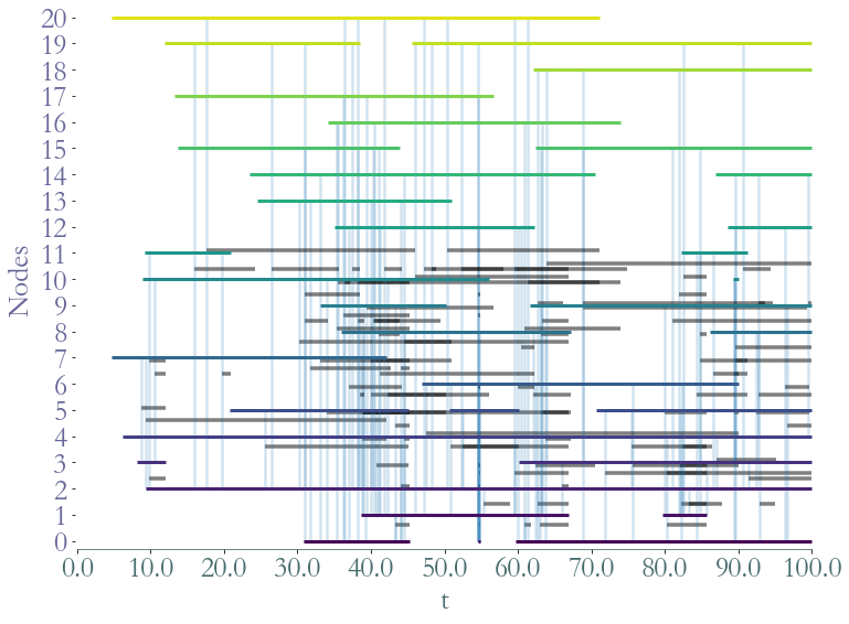
To plot the stream graph we use Straph’s custom function.

[6]:

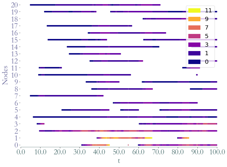
_ = S.plot()
_ = S.plot(clusters = S.degrees_partition(),plot_links=False)

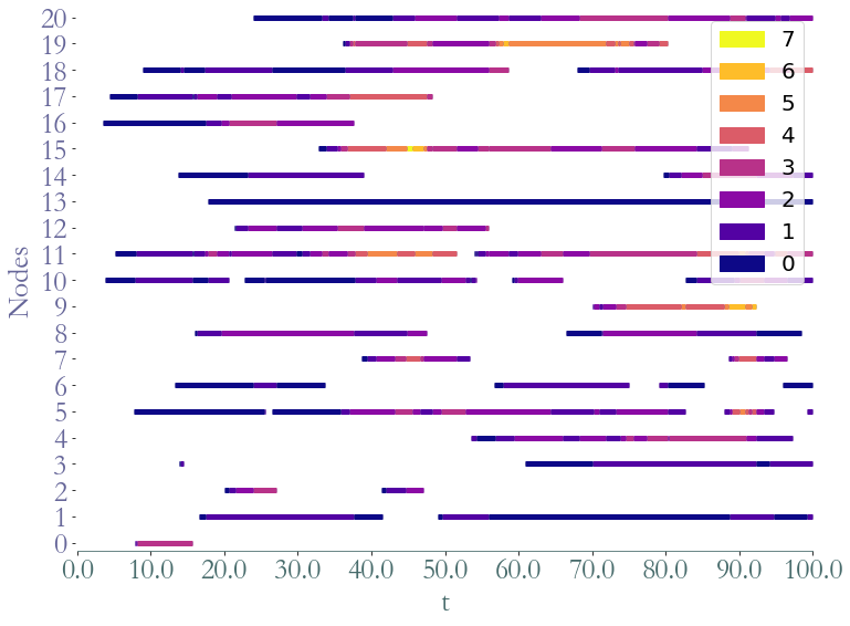
../_images/notebooks_Random_Stream_Graphs_12_0.png

../_images/notebooks_Random_Stream_Graphs_12_1.png

Degree distribution¶

[7]:

T = [0, 1000]
nb_node = 3000
occurrence_law_node = 'poisson'
presence_law_node = 'uniform'

occurrence_param_node = 4
presence_param_node = 100

occurrence_law_link = 'poisson'
presence_law_link = 'uniform'

occurrence_param_link = 4
presence_param_link = 50


p_link = 2*numpy.sqrt(nb_node)/nb_node

S = sg.erdos_renyi(T,
                    nb_node,
                    occurrence_law_node,
                    occurrence_param_node,
                    presence_law_node,
                    presence_param_node,
                    occurrence_law_link,
                    occurrence_param_link,
                    presence_law_link,
                    presence_param_link,
                    p_link)


                                    

If we observe the degree distribution of these random stream graph we observe the same distribution as in erdos-renyi static graphs.

[8]:

degrees = S.degrees()
_ = sg.hist_plot(list(degrees.values()), xlabel = "Nodes Degree", bins = 20)

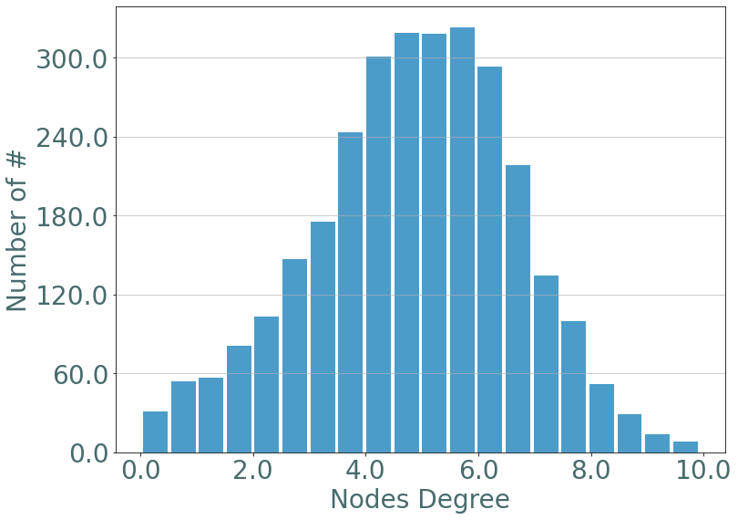
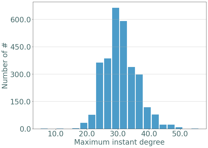
../_images/notebooks_Random_Stream_Graphs_16_0.png

If we plot the maximum instant degree we observe the same distribution as in erdos-renyi static graphs.

[9]:

d_part = S.degrees_partition()
max_d = {}
for d, v in d_part.items():
    for u in v:
        max_d[u[2]] = d

_ = sg.hist_plot(list(max_d.values()), xlabel = "Maximum instant degree", bins = 20)

                                    

../_images/notebooks_Random_Stream_Graphs_18_0.png

Barabasi Albert¶

As in static graph our Barabasi-Albert takes two parameters m0 the initial number of nodes and m the number of nodes that will be connected to a new node.

[10]:

T = [0, 100]
nb_node = 21
occurrence_law_node = 'poisson'
presence_law_node = 'uniform'

occurrence_param_node = 3
presence_param_node = 25

occurrence_law_link = 'poisson'
presence_law_link = 'uniform'

occurrence_param_link = 5
presence_param_link = 15


m0 = 3
m = 3

                                

[11]:

S = sg.barabasi_albert(T,
                    nb_node,
                    occurrence_law_node,
                    occurrence_param_node,
                    presence_law_node,
                    presence_param_node,
                    occurrence_law_link,
                    occurrence_param_link,
                    presence_law_link,
                    presence_param_link,
                    m0,
                    m)
S.describe()

                                

Nb of Nodes :  21
Nb of segmented nodes :  35.0
Nb of links :  55
Nb of segmented links :  114.0
Nb of event times :  202

[12]:

_ = S.plot()
_ = S.plot(clusters = S.degrees_partition(),plot_links=False)

../_images/notebooks_Random_Stream_Graphs_23_0.png

../_images/notebooks_Random_Stream_Graphs_23_1.png

Degrees Distribution¶

[13]:

T = [0, 1000]
nb_node = 2000
occurrence_law_node = 'poisson'
presence_law_node = 'uniform'

occurrence_param_node = 4
presence_param_node = 100

occurrence_law_link = 'poisson'
presence_law_link = 'uniform'

occurrence_param_link = 4
presence_param_link = 50


m0 = 10
m = 4

                                    

[14]:

S = sg.barabasi_albert(T,
                    nb_node,
                    occurrence_law_node,
                    occurrence_param_node,
                    presence_law_node,
                    presence_param_node,
                    occurrence_law_link,
                    occurrence_param_link,
                    presence_law_link,
                    presence_param_link,
                    m0,
                    m)
S.describe()

                                    

Nb of Nodes :  2000
Nb of segmented nodes :  5639.0
Nb of links :  6416
Nb of segmented links :  11356.0
Nb of event times :  24682

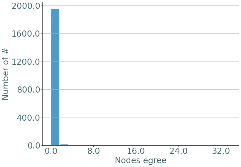
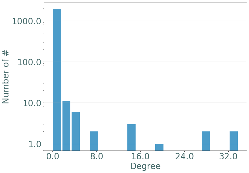
If we observe the degree distribution of these random stream graph we observe the same distribution as in barabasi-albert static graphs.

[15]:

degrees = S.degrees()
_ = sg.hist_plot(list(degrees.values()), xlabel = "Nodes egree", bins = 20)

../_images/notebooks_Random_Stream_Graphs_28_0.png

We add a logscale on the number of values:

[16]:

_ = sg.hist_plot(list(degrees.values()), xlabel = "Degree", bins = 20,ylog = True)

                                    

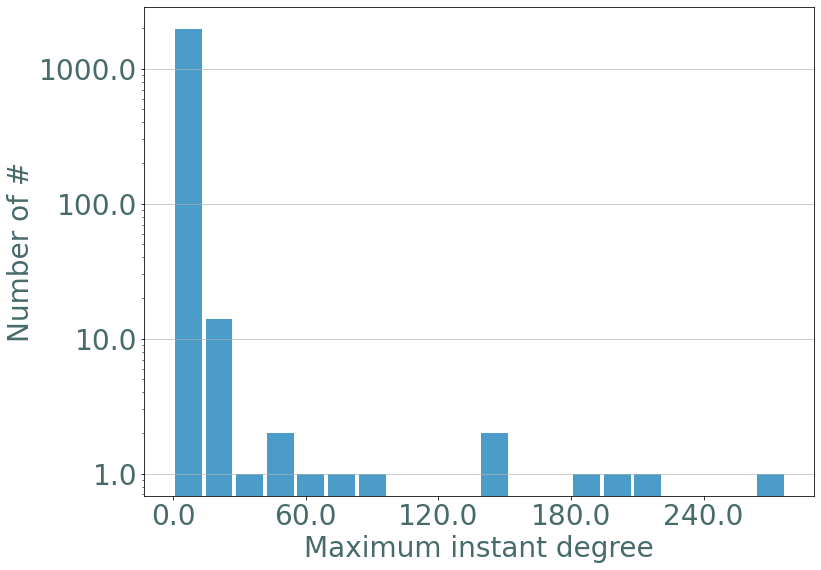
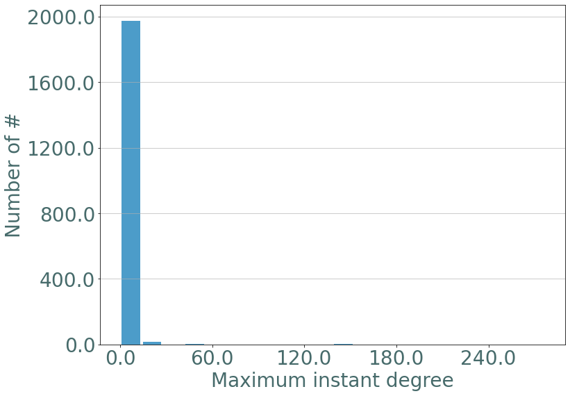
../_images/notebooks_Random_Stream_Graphs_30_0.png

Similarly with the maximal instant degree:

[17]:

d_part = S.degrees_partition()
max_d = {}
for d, v in d_part.items():
    for u in v:
        max_d[u[2]] = d
fig = plt.figure()
_ = sg.hist_plot(list(max_d.values()), xlabel = "Maximum instant degree", bins = 20)

                                    

<Figure size 864x648 with 0 Axes>

../_images/notebooks_Random_Stream_Graphs_32_1.png

[18]:

_ = sg.hist_plot(list(max_d.values()), xlabel = "Maximum instant degree", bins = 20, ylog = True)

                                    

../_images/notebooks_Random_Stream_Graphs_33_0.png

Temporal Paths in Stream Graph Temporal Network Analysis: High School Dataset, Interactions among Students